
Let’s reduce the number of tests (experimental design method)
We try to figure out combinations of several conditions for testing for quality and purpose extraction. If it is a normal idea, if you do the number of rounds per minute (by testing) it is certain. , but in cases where there are many types of combination conditions or there are many condition contents, the number of brute force increases exponentially. (It increases the number of tests.) It becomes way to suppress it as much as possible.
Rather than doing the number of experiments by round robin, express by probability · Reduce the number of times by performing with probability
Difference from brute force
Suppose, for example, you want to investigate the best condition under the condition that the seed of the plant germinates. Tentatively, as the type of condition, “type of soil” “quantity of water”. As the content of the condition, the brute force in the case of “type of soil” is “red soil”, “black soil”, “normal soil”, “the amount of water” is “less than 100 ml” “100 ml or more and less than 500 ml” or “500 ml or more” The number of times and the table (combination pattern) are as follows.
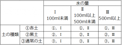
The round-trip count (test count) is 3 × 3 = 9 times .
I will increase the type of condition here by one. The type of condition is “temperature”, the contents of the condition is set to “less than 10 ° C”, “10 ° C to 20 ° C”, “20 ° C or more”. In this case, the total number of contacts and the table are as follows.
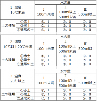
The round-trip count (test count) is 3 × 3 × 3 = 27 times . It increases steadily with a multiplier. . .
However, If it is the idea of the experimental design method, the number of times of experiments is not required for the total number of rounds. What are you talking about? You might think. It is represented in the table below.
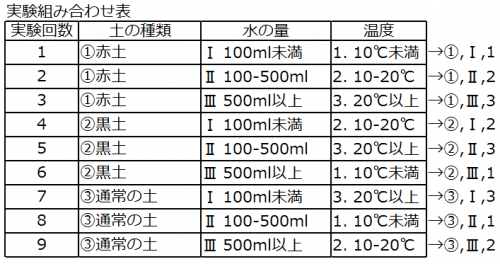
I think that I thought that “There is a pattern that is not done !!” ! In the experimental design method, the proportion of the contents (large elements) of the related condition is given using the analysis method of variance analysis. To put it briefly, a technique for establishing relevance by establishing it . Therefore, we have to compute the result. . . If you make it in Excel etc. beforehand, it is no problem.
Benefits:
The number of tests decreases. The relevant ratio of the contents of the condition can be specified.
Demerit:
The best combination is hard to understand, calculation is necessary
(You can see which items are strongly related by the content of each condition.)
Two things can be analyzed by using the experiment design method.
1. Reducing the number of tests: It will also be the subject of the title.
2. Analysis of data: You can tell by the probability how much the condition contents are related.
Concept of experiment design method
In the experimental design method, the type of condition mentioned earlier is called “factor” and the content of condition is called “level”.
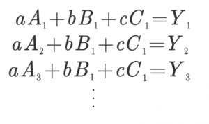
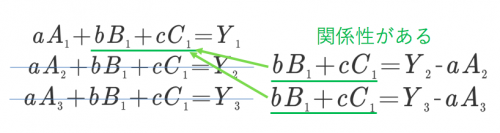
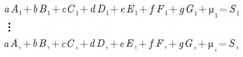
I think that we can write the factors A, B, C and the levels 1, 2, 3 (A1, A2, A3) as calculation formulas as follows when thinking in brute force.
It is not simple, but I will briefly explain.
· way of thinking
Among the above formulas, I think you will find that there are related parts (common parts) when rewritten as follows.
Even if you do not conduct a direct test using this relationship, the test results will appear in the common part so that it is a way to be tested without testing the whole number. Originally I will think about dispersion (variation).
Therefore, combination is very important . The combination uses an orthogonal table derived from a table called Latin square. It will be a combination called. By using the orthogonal table, the effect of each factor can be evaluated without counting in round robin (even without combining all patterns). This combination is important.
· What is Latin square?
If you explain the Latin square in a simple way, it arranges so that one element is inserted in each row. Use it to spread the combination.
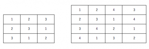
An orthogonal table is obtained by weighting the variance using this Latin square.
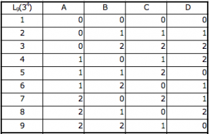
The following is an orthogonal table to be used in this case.
The idea is difficult ~! Well, I am the same.
The theory is difficult, but If you apply the correct pattern as it is, there is no problem.
For those who want to know more, the following books will be helpful.
Next we will show the orthogonal table to use.
The important thing is just to assign an orthogonal table to use, depending on what level / factor / you want to do .
Reduce the number of tests by utilizing the fact that the test results appear in the common part.
Orthogonal Table Type
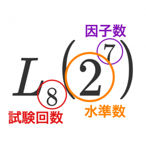
First of all, it is the notation method before showing the kind.
Write it as orthogonal table as follows.
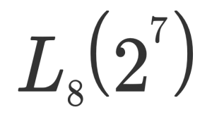
What’s this? However, this means that two levels of factors are orthogonal tables that can be handled up to 7 tests in 8 tests.
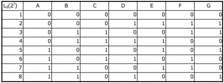
Orthogonal table: 2 levels 3 factors
Orthogonal table: 2 levels 7 factors
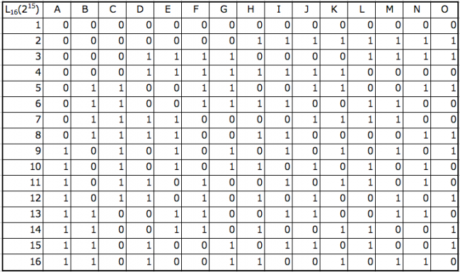
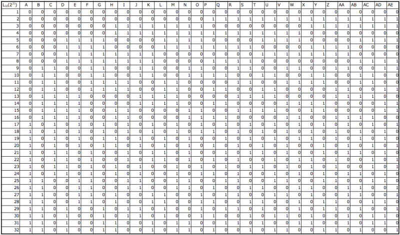
Orthogonal table: 2 levels 15 factors
Orthogonal table: 2 levels 31 factors
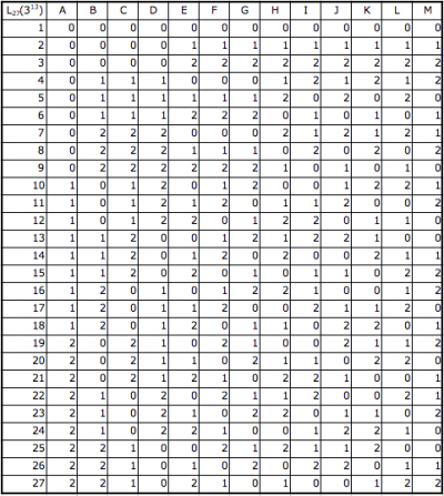
Orthogonal table: 3 levels 4 factors
Orthogonal table: 3 levels 13 factors
If the number of factors to be used is small, please use the factor without assigning any factors that have the remainder of the orthogonal table.
I presented a representative one. There are many others and it is also possible to derive.
There are combinations of levels (combination of 2 levels and 3 levels, etc.) and multiple levels of orthogonal tables, but we will skip here.
For details, please see the reference material at the end of the sentence.
After all, let’s try to minimize as much as the number of factors / level number increases as the number of experiments increases.
There are various kinds
Minimize the factor / level to conduct the test
How to evaluate in Excel
I think that I understood the kind of the orthogonal table. I will explain concretely how to use it.
Evaluation of Pass Rejection
In this state, we know the value of the acceptance and we will put out the completeness of the combination.
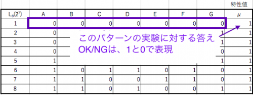
First select the orthogonal table you want to use. Here we use an orthogonal table of 8 tests (2 levels 7 factors).
As mentioned earlier, even if the number of factors is small (in this case two factors, six factors can be used).
In that case, please ignore the column (column).
· Thinking (pass failed)
As a way of thinking, we solve the following simultaneous equations.
Compare the characteristic value (predicted value, average value) μ with the result S and see the change in the coefficients a to g.
If the characteristic value and the result are the same, the coefficient becomes 0. Changes appear in the coefficients involved when they are different.
· How to use Excel (pass fail)
First, we will output the necessary orthogonal table. Add the column of the experimental characteristic value (predicted value, average value) μ to the last column of the orthogonal table.
For 2 pole like OK / NG for characteristic value, indicate it with 1 and 0.
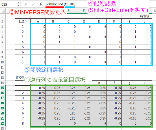
First, create an inverse matrix to solve the simultaneous equations.
In Excel, we use “MINVERSE function”.
① Select the same range as the orthogonal table + characteristic value range for the place you want to create the inverse matrix (the place you want to display).
② Fill in MINVERSE in the input field.
③ Select the range of MINVERSE (what you want to inverse matrix: orthogonal table + characteristic value).
④ I will let Excel recognize it as an array. In Excel, “Shift + Ctrl + Enter” will be recognized as an array that is related not to a simple numerical value.
This completes the inverse matrix table.
This time, it performs matrix multiplication and displays the change of coefficients a ~ g.
In Excel, we use “MMULT function”.
① Select the range of the number of factors plus 1 (characteristic value) in the same way as above, where you want to make the matrix product (the place you want to display).
② Fill in MMULT in the input field.
③ Select the range of MMULT (what you want to matrix, orthogonal table + inverse matrix of characteristic value, result).
④ I will let Excel recognize it as an array. In Excel, “Shift + Ctrl + Enter” will be recognized as an array that is related not to a simple numerical value.
This completes the matrix product table (values of coefficients a – g).
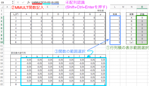
You can see which factors are related from these.
· It can be said that factors with a change in the evaluation (coefficient) have influence (change) on the characteristic value.
Of course, if the characteristic value and the result are exactly the same, the evaluation (coefficient) will be 0.
In the case of evaluation such as pass fail, it means that it is a failure if the evaluation is other than 0.
As a factor of rejection, if the characteristic value (acceptance value) is 1, a negative factor of evaluation is a factor.
In this case, it can be said that factors of E and G cause this result to be different from the characteristic value.
Evaluation judgment and relevance of factors can be judged by Excel
If you prepare a calculation formula in Excel in advance, you can easily find related factors
Evaluation of maximum or minimum combination estimation
Here, we will explain how to find out which combination the numerical value is the maximum or minimum.
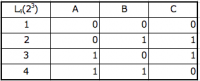
First select the orthogonal table you want to use. Here we will use orthogonal tables (2 levels 3 factors) of 4 tests.
· Concept (combination estimation)
We will use the orthogonal table to obtain the evaluation value.
Assign the result to the level of each factor.
Divide the factor by the number of allocated results of that factor and level and compare it.
If there are multiple test results, errors in measurement are suppressed and accuracy improves.
At that time, if the test result is D, the relationship between the true measured value S and the error N is as follows.
D = S + N
If it is 1 time, this is fine, but if you do it more than once, you will see the error on average as you try to express it on average.
Assuming that the test result is 3 times (D1, D2, D3) the average value D of the test, it can be expressed as follows.
/ 3 = S + (N 1 + N 2 + N 3) / 3 (S 1 + N 2 + D 3) / 3 =
If the error is close to the true measured value, it is difficult for the error (variation) to understand the difference between the true measured values by just normal means alone.
So it is the idea of dispersion.
We will give the expected value of variance of sample mean.
σ ^ 2 = (D1 ^ 2 + D2 ^ 2 + D3 ^ 2) / 3 = (Measurement 1st ^ 2 + Measurement 2nd ^ 2 + Measurement 3rd ^ 2) / 3
This variance value itself does not make sense, but if the error is even slightly less than the true measurement value, the true measured value is largely reflected.
“When the result of the test is multiple (n times)”, because the variance itself is raised to the second power, digits of the value are sometimes enlarged and it may be difficult to see, so we use LOG to reduce the scale.
The error (variation) is explained in “Variance and process capability” .
· When the test result is single (once)
I will explain the case where there is only one result for the number of tests.
Actually, since there is noise (variation), the number of tests will be reduced by the experimental design method but the test result will be more accurate if you do multiple tests.
Later, I will explain the case where multiple results are issued, but here we will explain the result one time.
In this example, we will find combinations (combinations of factors and levels) that maximize the test results.
We will use an orthogonal table of 2 levels 3 factors as below and take the results once (4 in total) for 4 test times (4 patterns).
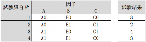
With this list of test counts in order, rearrange the test order and test results of each factor as follows.
As you can see from the table, we just assigned the test results to the factor test order.
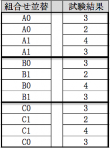
After that, we will issue total test results at the level of each factor.
Also we will count the number of factors that each level of factor has come up in the test.
Because of the test combination of the orthogonal table, the number of items appearing in the test of the level of each factor differs depending on the table.
We take an average and estimate the level value of each factor.
Since we want to find the maximum combination here, the highest combination of levels of each factor of the largest numerical value becomes.
(If you want to obtain the minimum, the combination with the smallest level of each factor is the combination with the smallest level.)
The maximum combination here is “A1, B0, C0” or “A1, B0, C1”.
Even if you use a different orthogonal table it is possible to do the same.
· When the test result is multiple (n times)
I will explain the case where multiple results are output for the number of tests (when multiple measurements are taken).
As I mentioned earlier, since there are errors in practice, the number of tests will be reduced by the experimental design method, but the test results will be more accurate if you do multiple tests a few times.
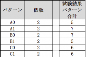
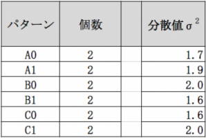
We use three factor 2 level orthogonal table as below and take 3 results (total of 12) for 4 test times (4 patterns).
It is the same as halfway “When the test result is single (once)”.
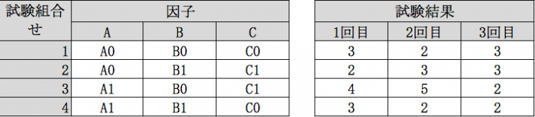
With this list of tests in order, distribute the test order of each factor and three test results and rearrange them as follows.
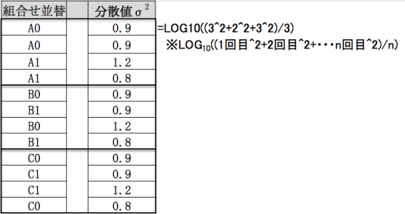
As I mentioned earlier, we will give the expectation of sample variance from test results.
Dispersion (σ 2) = (first test result ^ 2 + … + n th test result ^ 2) / n
Here we are logarithm using LOG.
When using Excel, try using the function “LOG 10”.
In sorting you can see by looking at the table, but the dispersed test results are only repeating for each factor.
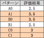
After that, we will make a total variance at the level of each factor.
Also we will count the number of factors that each level of factor has come up in the test.
We take an average and estimate the level value of each factor.
Since we want to find the maximum combination here, the highest combination of levels of each factor of the largest numerical value becomes.
(If you want to obtain the minimum, the combination with the smallest level of each factor is the combination with the smallest level.)
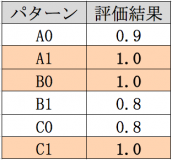
The maximum combination here is “A1, B0, C1”.
Likewise, even if you use a different orthogonal table, you can do it in the same way.
The largest combination can be easily estimated with Excel
Points to note in testing
Although it is not limited to this, attention is required for measurement in the test.
It is to make sure that data is not going wrong due to bias of conditions. For example, in the case of experiments such as those measured by humans, elements other than logical, such as preconceptions and memorization of previous data values, may be included. By doing it in random order, you can reduce those factors.
1. Measure several times
Measure several times to suppress variations in measured values. However, it can be omitted if the result does not vary.
2. Constant content other than factors
In order to limit to only the factors that become the condition, the external factor must be constant at all times.
3. Do in a random order
It is necessary to do it in random order to eliminate accustomment and prejudice to the examination.
Although the number of tests can be reduced, efforts to minimize external factors other than factors / levels are required
Experiment planning method in the field of economics (conjoint analysis)
The factor is called an item, and the level is called a category. Basically, with the same idea, I figure out what kind of element (the category in the item) is the strongest.
Since the way of thinking is the same as the explanation explained, we omit it.
Although it is not an exam as it was explained so far, it will be a method of making judgment using the data you have.
Up until now, the goal was to reduce the number of experiments.
For conjoint analysis, it is used to see how much the factor (the element here) is related as explained in Excel.
It is used in various fields other than economics. The name is variously different. . .
In addition to reducing the number of experiments, we often use it to see relationships like conjoint analysis.
· Analysis of factors and causes (confirmation of relevance of elements)
· Test for product defect check
It is used for element judgment and result judgment stochastically in various fields.
The experiment design method is performed when the relation of the element is not known. For that reason, we do experiments with content that understands relevance, which makes it much more troublesome. (I think that it is good in terms of confirmation) I think that there is a part that the expert in that field “knows somehow” that the relevance is related and it is said that it is said to be an experience · kang etc I will. Let’s use it for various things.
For those who want to learn more, this book is helpful.
Partial addition 2017/03/30